THE PERFORMANCE OF THE EPSILON AND THETA CONVERGENCE ACCELERATION ALGORITHMS

A Paper

Submitted to the Graduate Faculty

of the

North Dakota State University

of Agriculture and Applied Science

Paul Scott Heidmann

In Partial Fulfillment of the Requirements

for the Degree of

MASTER OF SCIENCE

Major Department:

Mathematics

August 1992

Fargo, North Dakota

THE PERFORMANCE OF THE EPSILON AND THETA CONVERGENCE ACCELERATION ALGORITHMS

Paul Scott Heidmann

The Supervisory Committee certifies that this paper complies with North Dakota State University's regulations and meets the accepted standards for the degree of

MASTER OF SCIENCE

SUPERVISORY COMMITTEE:

___________________________________________________________________

Chair

___________________________________________________________________

Approved by Department Chair:

___________________ __________________________________

Date Signiture

Abstract

Heidmann, Paul Scott, M.S., Department of Mathematics, College of Science and Mathematics, North Dakota State University, August 1992. The Performance of the Epsilon and Theta Convergence Acceleration Algorithms. Major Advisor: Associate Professor Davis Cope.

Motivations for transforms are first presented, along with the derivation of both the -algorithm and the -algorithm. Known properties are then presented, with a partial classification of the sets for which the transforms are known to have accelerative properties.

Empirical evidence is given illustrating the performance of the algorithms over a broad set of test series. The -algorithm was found to perform better than the -algorithm on all but a few of the test cases considered. No algorithm considered demonstrated any evidence of producing an increase in the exponential rate of convergence. No evidence of instability was seen among the algorithms considered.

Abstract................................................................................................................................ iii

Section 1: Introduction........................................................................................................... 1

Section 2: Transform Motivations and Properties.................................................................... 4

The Motivation of the e Transform................................................................. 4

Properties of the e Transform......................................................................... 7

The e Transform and the -Algorithm........................................................... 10

The Motivation of the q Transform............................................................... 13

Properties of the q Transform....................................................................... 14

Section 3: Empirical and Related Results.............................................................................. 16

Details of the Test Program.......................................................................... 17

Details of Test Procedures........................................................................... 17

Transform Singularities................................................................................. 18

Empirical Results......................................................................................... 23

Group 1.......................................................................................... 23

Group 2.......................................................................................... 77

Group 3.......................................................................................... 80

Group 4.......................................................................................... 95

Group 5........................................................................................ 101

Group 6........................................................................................ 115

Group 7.....................................................................................117

Section 4: Summary........................................................................................................... 126

Bibliography...................................................................................................................... 127

Section 1 Introduction

This paper is concerned with the evaluation of the performance of the -algorithm and the -algorithm when applied to sequences of partial sums. Transform definitions and properties are first stated, followed by empirical examples illustrating the comparative performance of the algorithms on a wide variety of test problems.

The two transforms covered in this paper are recursive and operate on the set of complex valued nonconstant sequences. For broad classes of sequences, these algorithms are known to have accelerative properties.

Both algorithms are actually more accurately described as a hierarchy of transforms. That is, the algorithms provide a succession of transforms, with the higher order transforms typically providing greater rates of acceleration.

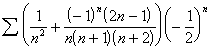
The first of these algorithms, the -algorithm, is defined as follows for any nonconstant sequence [6, p. 225]:

The second algorithm considered in this paper is the -algorithm, defined as follows for any nonconstant sequence [6, p. 225]:

In most practical applications, a transform must have the properties of regularity and of convergence acceleration. This paper was concerned more with the latter than the former; however, both definitions will be required.

Definition: A transform T is said to be regular for a convergent sequence s_n if

Definition: A transform T is said to accelerate the convergence of a sequence s_n if

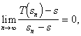
where s is the limit of the sequence s_n.

Intuitively, a transform accelerates the convergence of a sequence if the convergence of the transformed sequence is of higher order than that of the original sequence. Equivalently, a transform accelerates the convergence of a sequence if the error term of the transformed sequence asymptotically goes to zero with a higher order than the error term of the original sequence.

Section 2 of this paper summarizes the known properties of the transforms. The transforms are first motivated, and then theorems concerning each are presented.

Section 3 presents two new lemmas and presents the empirical research done in connection with this paper.

Section 4 summarizes the results reached in Section 3.

Section 2

Transform Motivations and Properties

The Motivation of the e Transform

The history of the e transform is not altogether clear. The general ideas which underlie this transform go at least as far back as Jacobi. A special case of the e transform known as the -process is usually attributed to Aitkin; however, this technique can be traced back to Kummer (1837) [8, p. 120]. Apparently, it was developed independently by several authors (although not always in its most general form): Delaunay, Samuelson, Shanks and Walton, Hartee, and Isakson [5, p. 5].

The e transform has been motivated by two distinct but similar sets of ideas. Both begin with the recognition that many sequences in applied mathematics and physics can be approximated by a limit together with exponential transients:

Here, it is assumed that none of the 's are zero or one (if a transient were one, it would become part of the limit s) and that the 's are distinct. The elemental idea is to develop a transform which will eliminate these exponential transients.

The first method of accomplishing this task was given by Shanks [5, p. 7-8] and is summarized below. Observe that any nonsingular sequence (definition follows) can be expressed as a kth order transient locally. Fix any n larger than k and represent as follows:

where the 's are the respective limits, called the "kth order local bases." Should one of the , then the sequence will be singular.^[1] These bases will vary relatively little as long as is nearly kth order [5, p. 7]. This fact suggests that the sequence of 's (for some fixed k) might converge faster than the sequence itself. This sequence of kth order local bases is then defined as the -transform of the sequence [5, p. 8], [in fact, it is identical with as defined in the following discussion.]

The motivation for the e transform given by Wimp [8, p. 121-123] also begins with the recognition that many sequences from applied mathematics and physics behave as if they were a limit combined with exponential transients. As above, the e transform is then developed to eliminate these transients; the technique by which the transform is developed, however, differs significantly.

To begin (as above), assume the sequence has the form:

To simplify notation, let:

Since is a linear combination of k exponentials, there is a linear difference operator of order k that annihilates :

( not zero).

Now, rewrite as follows:

Next, substitute into the difference equation, and solve for .^[2] Redefining constants gives:

This is a homogeneous system of equations with a nonzero solution . Such a solution will exist if and only if the following determinental equation is satisfied:

For simplicity, define:

Then, solving for s gives [8, p. 122]:

While the above equation will only be valid for sequences that can be represented as a combination of a limit and exponential transients, it can nevertheless be used to define a transform useful for a much larger class of sequences, which is written .

While these two derivations are quite different, they are indeed equivalent [5, p. 2-3,7-8].

Properties of the e Transform

At this point, several questions naturally arise. Questions concerning the regularity of the transform, the accelerative properties, and optimality are especially significant. This section presents known results that address these questions.

The first question that must be answered before the e transform can be used in any application is whether or not the transform will be regular for the sequences involved. For many applications, this question will not be difficult to answer, as the e transform can be shown to be regular on broad classes of sequences.

The following theorem (accredited originally to Lubkin) is stated by Shanks [5, p. 13]:

Theorem: If and both converge, then

Further regularity results are available for this transform and are discussed in the -algorithm section.

Closely related to the question of regularity is the question of exactness. That is, for what class of sequences will the e transform be exact (produce the limit of the sequence in a finite number of steps)? This question is answered in part by the following theorem, given by Shanks [5, p. 22]:

Theorem: Let f(z) be a rational function, which when reduced to its lowest terms has a q'th degree numerator and a p'th degree denominator; then, if

where is the first n terms of the Taylor expansion for f.

In fact, a closely related but stronger theorem has been given by Wimp [8, p. 125]:

Theorem: is defined for all and if and only if satisfies a homogeneous linear difference equation of order k with constant coefficients (and no equation of lower order) and contains no terms that are purely algebraic..

Finally, questions of optimality and accelerative properties must be addressed. Here, while fewer results are known, it is still possible to partially characterize sequences for which e is accelerative. A definition along with two helpful theorems are stated:

Definition: Let be the terms of a convergent series with partial sums and sum S. Let , and suppose that the sequences converge to , respectively. The convergence of the series is said to be logarithmic if , linear if , and of higher order if [6, p. 224].

The following two theorems are very useful for determining whether or not the condition is satisfied:

Theorem: If is of constant sign, then [3, p. 26].

Theorem: If with and if r is not -1, then [3, p. 26].

Wimp has shown [8, p. 104] that will accelerate all linearly convergent series. More interesting, however, are the results produced by Delahaye. Three basic results concerning the optimality of the transform (Aitkin's process) on the family of linearly convergent series are presented [4, p. 213]:

1. The transform is algebraically optimal; that is, it is not possible to find an algebraically simpler transform to accelerate the family of linearly convergent series.

2. It is impossible to accelerate the linear family with degree^[3] greater than 1, the degree of acceleration achieved with the transform.

3. The linear family cannot be enlarged into another accelerable family. That is, there does not exist a family of sequences containing the linear family for which can be shown to have the above properties.

Delahaye then interprets these facts [4, p. 213]:

These results do not mean that the is the best algorithm of acceleration. They only mean that concerning the family Lin, it is impossible to find a simpler or a more efficient algorithm of acceleration. This does not contradict the existence of subfamilies of Lin accelerable with degree 2, nor does it contradict the existence of algorithms less simple but equally efficient on Lin.

The e Transform and the -Algorithm

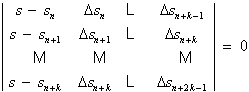
When first developed, the e transform was merely a curiosity. It had little practical value, as calculating the large order determinants inherent to the transform was computationally prohibitive. This changed in 1956 when Wynn produced the following theorem [9, p. 91]:

Theorem: If

and

then

provided that none of the quantities becomes infinite.

With this algorithm, it is now possible to compute the e transform easily and efficiently. Study of the -algorithm has also facilitated much knowledge of the e transform.

One such result is due to Wimp. However, before stating this result, two definitions are required :

Definition: A sequence s is totally monotone (written ) if

Definition: A sequence s is totally oscillatory (written ) if

[8, p. 12].

Theorem: Let the sequence s have remainder terms r; then, if r is either totally monotone or totally oscillatory, then is regular for all even m [8, p. 139 and 141].

While the algorithm is regular for large classes of sequences, this is not the only concern. Computing the transform involves repeated divisions by what can be very small quantities. This seems to suggest that the transforms will be prone to numerical instability. However, the empirical results presented in this paper suggest that the -algorithm is far more stable than appears at first.

Theoretical analysis of the stability of the -algorithm has not yet been fully developed. However, Wynn has presented a paper that begins to deal with this issue [10]. The results presented suggest that the -algorithm can be unstable for certain monotonic sequences [10, p. 110-112] and unconditionally stable for certain oscillating sequences [10, p. 112-115]. These theoretical results can be seen intuitively, simply by examining the transform. Oscillating sequences have adjacent terms opposite in sign. This tends to make the denominator in the defining recurrence relation larger. Monotonic sequences have terms of like sign, which in turn tends to make the denominator smaller.

Finally, the -algorithm can be shown to be closely related to the Padé table. The Padé table for an analytic function f is a two dimensional table of rational approximations of f. The [L,M] entry of the Padé table is typically denoted [L/M] and is defined as follows [1, p. 5]:

where is a polynomial of degree at most L and is a polymonial of degree at most M. The coeficients of the polynomials are chosen so that , where A(z) is the Taylor expansion of f(z) [6, p. 5]. If we require that Q and P have no common factors and that Q(0) = 1, then [L/M] is unique [1, p. 8].

The -algorithm produces certain entries in the Padé table. The following theorem then is due to Wynn [10, p. 93]:

Theorem: If the -algorithm is applied to the initial values

then

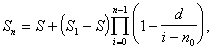
The Motivation of the Transform

The transform was developed by Brezinski as a means of accelerating the convergence of logarithmically converging sequences. Its motivation began with the observation that the algorithm fails to accelerate convergence on large classes of logarithmically converging sequences. However, rather than developing a completely new transform, Brezinski opted to modify the algorithm, adding an optimizing parameter.

Define . Then it is known that a set of sequences with logarithmic convergence having the property

may be accelerated by the algorithm modified with a "parameter of acceleration" [2, p. 727], specifically, with the following transform:

^[4]

A necessary and sufficient condition for to converge faster than is to take

However, calculating all of the parameters can be prohibitive. It was at this point that Brezinski took his departure from what was then known. His idea was to replace with the following approximation [2, p. 729]:

The transform then results.

Properties of the Transform

A property important in the application of any transform is regularity. Brezinski has characterized this property with the following theorem [2, p. 730]:

Theorem: For real valued sequences, a necessary and sufficient condition for

is that

As to the transform's accelerative properties, two theorems are given here. The first, and less general theorem, results from Germain-Bonne's theorem and is given by Smith and Ford [6, p. 225]:

Theorem: accelerates linear convergence.

The second theorem, due to Brezinski [2, p. 730], is much farther reaching:

Theorem: If is regular and if exists and is finite, then converges faster than .

Finally, the question of exactness is addressed by a theorem due to Cordellier and stated by Smith and Ford [6, p. 229]. It should be noted that this theorem characterizes only those sequences for which is exact in one term.

Theorem: for if and only if the sequence is one of the following three types:

1. where

2. where and neither is a positive integer.

3. and d is not a positive integer.

Section 3

Empirical and Related Results

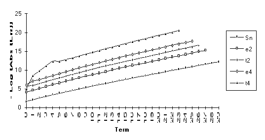
This section describes the empirical research done in connection with this paper. Many series^[5] were computed, and the transforms were applied to the sequences of their partial sums. The error terms for the sequences of partial sums, as well as the transformed sequences, were plotted. This allowed observations to be made concerning acceleration rates, stability, and unusual behavior (where it occurred).

Special software was constructed as arbitrary precision proved to be necessary. The high amount of precision was required for different reasons. Many of the transforms achieved upwards of 35 places of precision in only 30 terms. Other series were chosen to be very close to singular values for the transforms. Also, the high precision allowed elimination of numerical problems, so the properties of the transforms could be easily studied.

Details of the Test Program

This section describes the program used to perform the calculations involved in constructing the many examples presented in this paper.

As many precision problems can arise during the calculation of these transforms, arbitrary precision was necessary for the observation of the behavior of the transforms considered in this paper.

The storage of arbitrary length numbers was accomplished using linked lists. Specifically, the numbers were stored as linked lists of bytes, each byte containing two digits. Also, since the transforms operate on sequences, it was necessary to store sequences of these arbitrarily long numbers. This was accomplished in a similar manner, using linked lists. Finally, subroutines were added to perform arithmetic functions and transforms on these arbitrarily long sequences of arbitrarily long numbers.

Details of Test Procedures

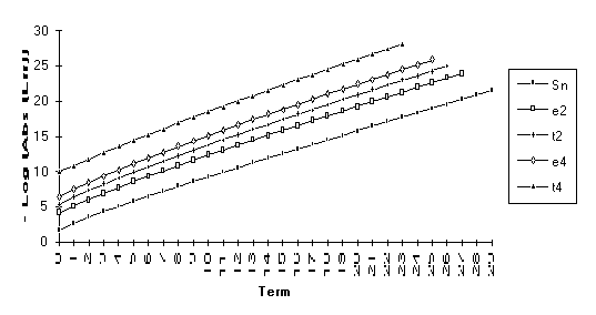
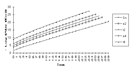
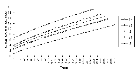
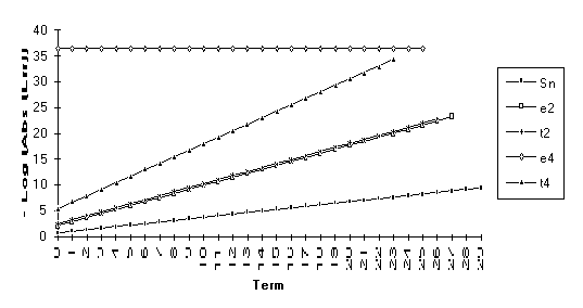
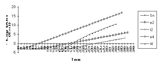
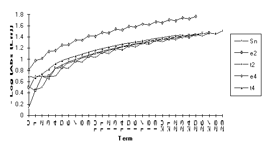
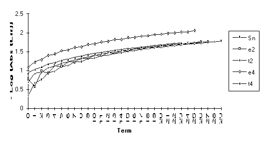
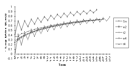
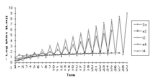
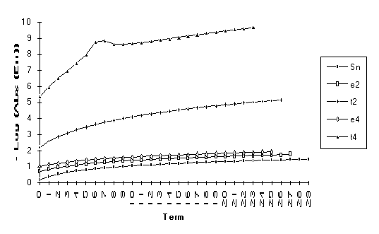
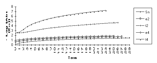
Following are several graphs illustrating the results of the empirical research done. All graphs are plots of the log (base 10) of the absolute value of the error. This configuration allows the approximate number of digits accurately calculated to be viewed at a glance.

The graphs contain two types of information. First, there is the size of the error term for each of the series and their transforms. Secondly, the rate of exponential acceleration can be seen in the slope of the corresponding line.

The actual value that any series under consideration converges to must be known. For those series which proved to have a reasonable rate of convergence, this limit was computed simply by summing the series out to several hundred terms before the transforms were computed. For those series with slower rates of convergence, Kummer acceleration was used to arrive at the limit. Several series had to be eliminated from the test set because their limit could not be computed.

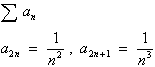
Many of the series contained a term . Where it was found, this modifier was defined as follows:

The 's provided a nonrational factor that did not change the value of .^[6]

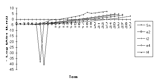
Transform Singularities

In this section, two lemmas are given that demonstrate that it is possible for the transforms to have singularities. Two illustrations are also be given to demonstrate the behavior of the transforms near a singularity.

Lemma: Apply the -algorithm to the sequence . Then, is undefined if .

Proof: From the defining equations,

However, since is a sequence of partial sums,

Combining the above,

This will be undefined whenever .

Remarks:

1. If the sequence in question is a power series of the form , then will be undefined at .

2. This result may be generalized to an arbitrary sequence . The n^th term of will be undefined when .

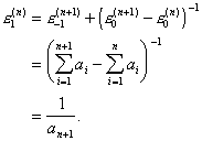
The following graph illustrates the above lemma. The numeric value used here was chosen to be very near to the value that would cause to be undefined. As can easily be seen, this sort of behavior cannot be ignored in practical applications of this algorithm.

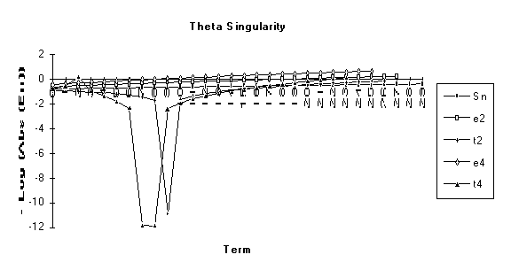
Analogously, a similiar lemma can be proven for the algorithm:

Lemma: Apply the -algorithm to the sequence . Then, is undefined if .

Proof: From the defining equations,

This will be undefined when .

Remarks:

1. If the sequence of partial sums is a power series of the form , then is undefined at .

2. This result may be generalized to an arbitrary sequence . In this case, is undefined if where .

The following chart illustrates the above lemma. The numeric value used here was chosen to be very close to the value that would make undefined. As before, this behavior cannot be ignored if the algorithm is to be used in practice.

Other examples of how these singularities affect the behavior of the transforms have been computed, but they are not included here as the behavior is the same in all examples considered.

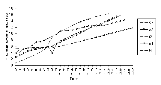
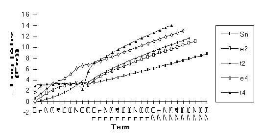
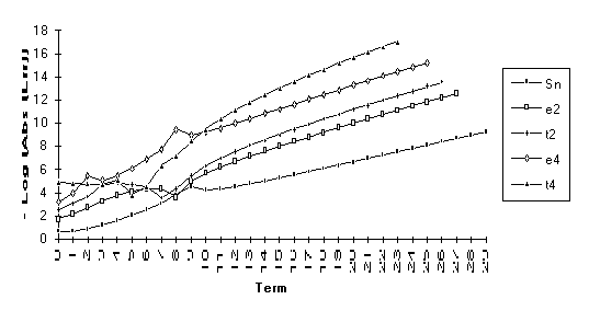
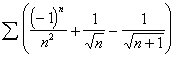
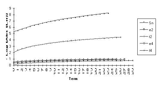
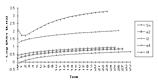
Empirical Results

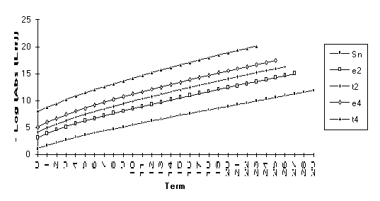
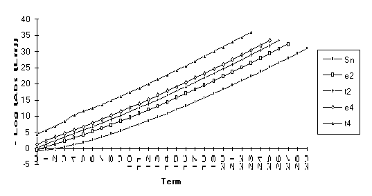
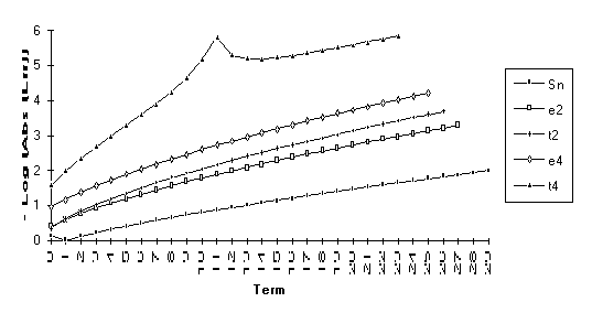
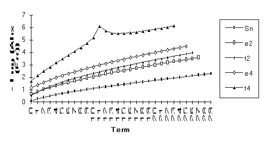
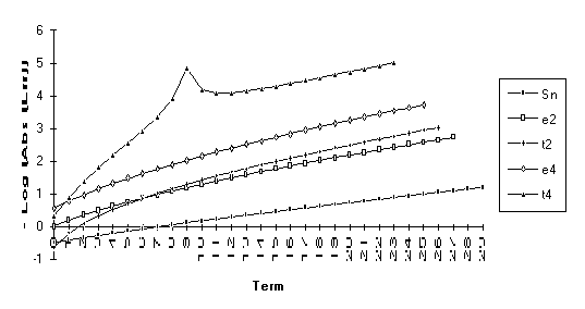
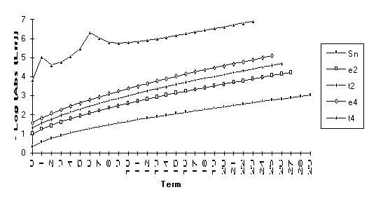
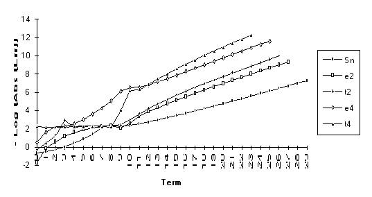
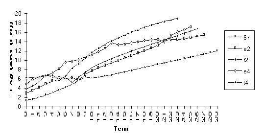
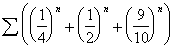
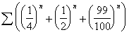
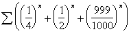
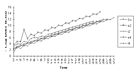
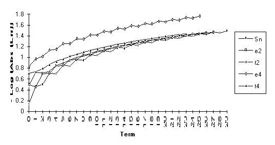
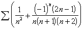
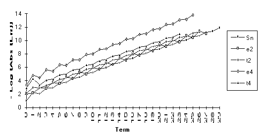
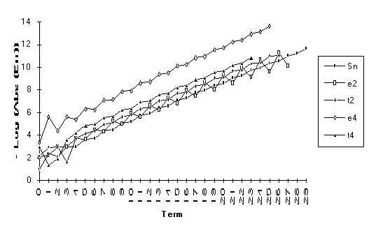
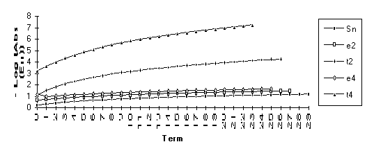
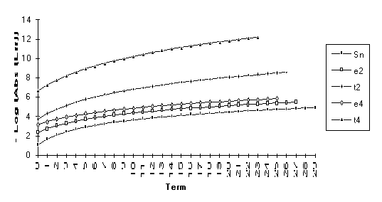
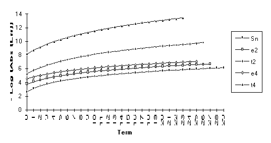
Group 1

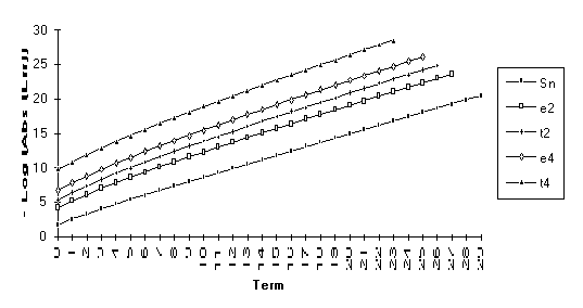
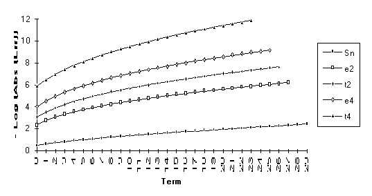
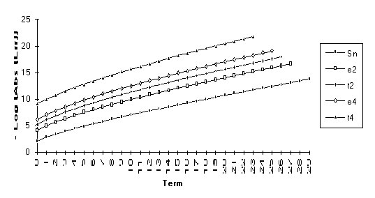
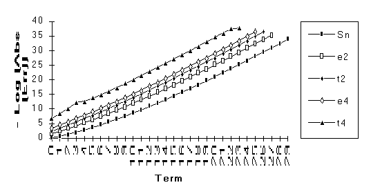
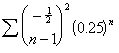
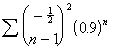
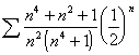
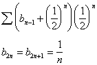
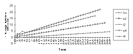
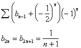
This set consists of those series for which the following order of performance can be clearly seen (from best to worst): . This is by far the largest group, suggesting that the -algorithm generally outperforms the -algorithm.

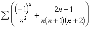
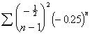
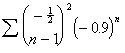
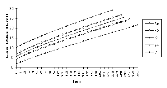
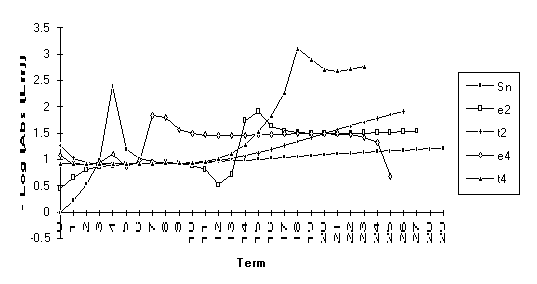
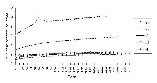
The anomoly in this graph is due to the fact that is nearly undefined (as discussed at the end of Section 3).

Note: Calculations made with 50 places of precision.

Note : The graphs of the transforms of this function have a significantly larger slope than the original series. This indicates a change in the exponential rate of convergence.

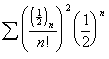
Group 2

This group contains series for which is exact. These series can all be shown to be a combination of a limit and two exponential transients. Notice that, for all of these series, the order of performance (from best to worst) is .

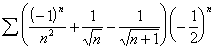
Group 3

This group contains series for which eventually outperforms , but otherwise the results are unclear. All series in this group contain the nonrational modifier .

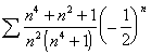
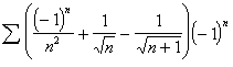
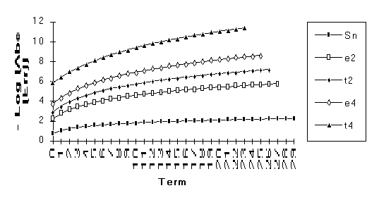
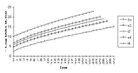
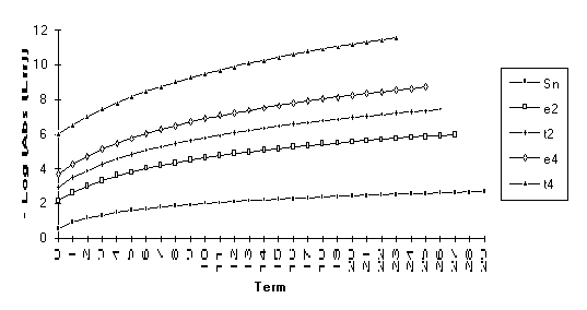
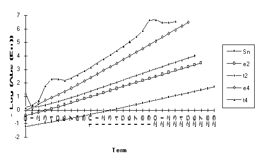
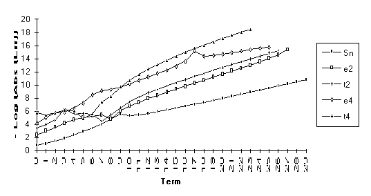
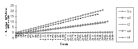
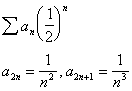
Group 4

This group contains the series for which the following order of performance is observed (from best to worst): . For all but the first series in this group, the -algorithm will eventually be exact.

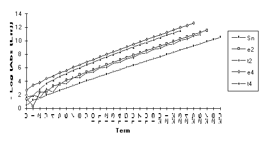
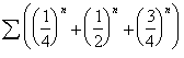
This sequence can be shown to be a combination of its limit and three exponential transients. The epsilon algorithm will then be exact by the sixth iteration. Notice here that the epsilon algorithm outperforms the theta algorithm. This is due to the fact that this is exactly the type of sequence that the e transform was designed to accelerate.

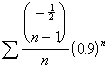
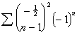
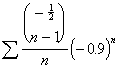
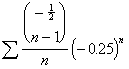
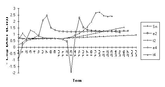
This and the next three series are included to demonstrate the effect of singularities on the transforms. All terms of both the -algorithm and the -algorithm are undefined at 1. The inclusion of the successive terms 0.9, 0.99, and 0.999 illustrates the continuing degradation of the algorithms as the singularities are approached.

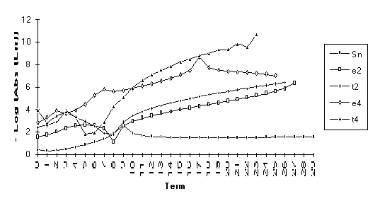
Group 5

This group of series bears the following peculiar attribute: only achieves any acceleration.

Note: For the above function, does not exist, but .

Note: For this series, 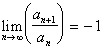, but does not exist.

Group 6

This group consists of a single series which none of the algorithms considered accelerated.

Note: For this series, , but .

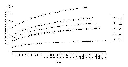
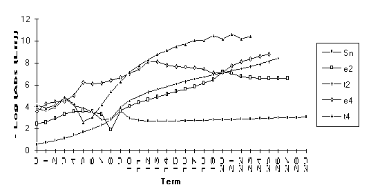
Group 7

For this group of series, the following order of performance is observed (from best to worst): .

Section 4

Summary

Several conclusions have been reached in this paper; this section summarizes these results. The two lemmas presented in Section 3 are worthy of special mention here. In any practical application of the algorithms addressed in this paper, it is critical to be aware of any anomalies that might occur. The graphs associated with the lemmas illustrated the profound effect a singularity can have on a transform.

In the series considered, outperformed except for a few cases.

There did not appear to be a change in the exponential rate of convergence between and unless otherwise noted.

No evidence of numeric instability was observed in any of the transforms considered (only in the case where a transform was nearly undefined could any instability be seen).

Bibliography

[1] Baker, George A., Jr.

Essentials of Padé Approximants

Academic Press, New York, 1975

[2] Brezinski, Claude.

Acceleration de suites a convergence logarithmique.

C. R. Acad. Sc. Paris, 18 October 1971, p. 727-730.

[3] Clark, W. D., Gray, H. L., Adams, J. E.

A Note on the T-Transformation of Lubkin.

Journal of Research of the National Bureau of Standards, B. Mathematical Sciences, Vol 73B, No. 1, January - March 1969, p. 25-29.

[4] Delahaye, Jean-Paul.

Sequence Transformations.

Springer-Verlag, 1980.

[5] Shanks, Daniel.

Non-Linear Transformations of Divergent and Slowly Convergent Sequences.

Journal of Mathematics and Physics, Vol 34, 1955, p. 1-42.

[6] Smith, David A., Ford, William F.

Acceleration of Linear and Logarithmic Convergence.

Journal of Numerical Analysis, Vol 10, No. 2, April 1979, p. 223-240.

[7] Smith, David A., Ford, William F.

Numerical Comparisons of Nonlinear Convergence Accelerators.

Mathematics of Computation, Vol. 38, No. 158, p. 481-499.

[8] Wimp, Jet.

Sequence Transformations and Their Applications.

Academic Press, 1981, p. 120-147.

[9] Wynn, P.

On a Device for Computing the e_m(S_n) Transformation.

Mathematical Aids to Computation, Vol. 10, 1956, p. 91-96.

[10] Wynn, P.

On the Convergence and Stability of the Epsilon Algorithm.

Siam Journal of Numerical Analysis, Vol. 3, No. 1, 1966, p. 91-122.

^[1]This would result in a division by zero when trying to solve for the local bases.

^[2]This requires that s_n not be a constant sequence.

^[3]A (regular) transform is said to converge more rapidly than a sequence with degree if for every there exists a natural number N such that for all n > N, where s is the limit of the sequence and of the transform [4, p. 129].

^[4]Brezinski calls this transform the transform and calls what we know as the transform the -transform. I have interchanged this notation to avoid confusion.

^[5]All series in the test set have the form .

^[6]Where the 's are the coefficients of the series in question.